Introduction
The regulation of transformers with tap changers is a classical subject within the field of power supply and distribution. Today these tasks are accomplished electronically with high regulation quality. Digital regulators, such as the freely programmable REGSys® voltage regulator system, are in use.
The core of the REGSys® voltage regulator system (Figure 1) is the REG-D® voltage regulator which, in addition to its actual regulating function, also performs measuring, recording and statistical functions. The parameterization of the regulator can be carried out menu-driven either directly via the keyboard or via PC with the help of WinREG software. The communication interfaces are of particular importance for parallel regulation. All of the relevant data can be exchanged via the E-LAN regulator bus with two interfaces (RS 485 interface), which enables data communication between up to 255 regulators. Expensive measuring supplements or parallel regulating units are therefore superfluous.
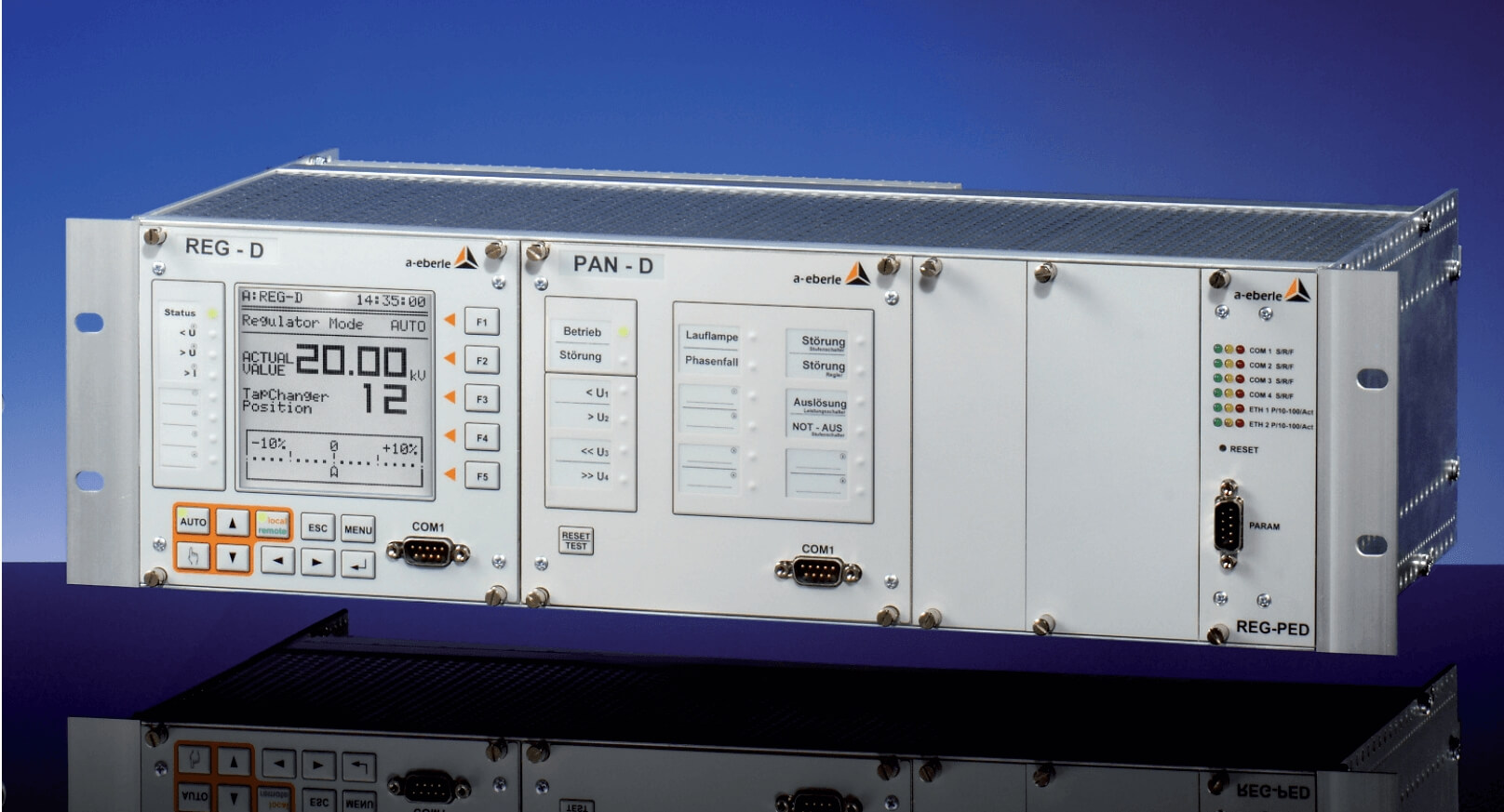
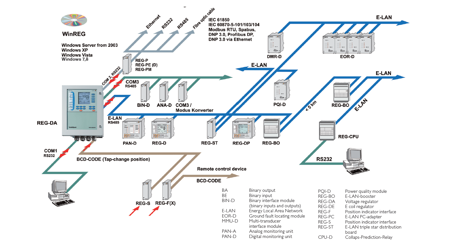
The COM 1, COM 2 (RS232) and COM3 (RS485) serial interfaces are used for linking the PC, the modem, the supplementary interface modules and the higher-level I&C. Analog and binary inputs and outputs are available for the most varied measuring and regulating functions involving the transformer. This makes it possible to implement, for example, tap position acknowledgement or a setpoint change over. The possibilities for expanding the system up to including Petersen coil regulation and ground-fault detection are illustrated in Figure 2.
Parallel transformer regulation with REGSys®
Although it is fairly easy to regulate an individual transformer, the conditions become confusing when operating in parallel. There are numerous reasons in favor of parallel transformer operation: The required power can be distributed to several transformers and, in the case of outages, reserves are available for providing the required electrical power. If several branch circuits are to be fed, the transformers can be connected in parallel to different busbars according to the power requirement in order to flexibly accommodate power peaks.
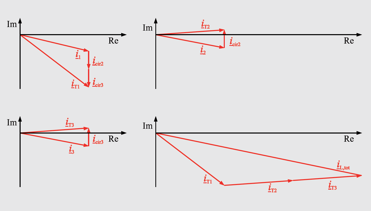
The parallel connection of n transformers is illustrated in the form of a substitute connection diagram in Figure 3. The diagram clearly reveals that special precautionary measures are necessary for parallel operation. If, for example, the source voltage u1 is higher than u2 to ux, the circulating currents icir2 to icirx will flow. The circulating currents are dependent on the short-circuit impedances Zsc1 to Zscx and the differences between the open-circuit voltages u1 – u2 to u1 – ux. Since the impedances of the transformers are normally very small, considerable circulating currents can flow if the transformers have been upset accordingly. In a borderline case, this could cause the transformers to be overloaded or to be at least unfavorably used to capacity. The following equations clarify the connections:
iT1 = i1 + icir2 +….+ icirx (1)
iT2 = i2 – icir2 (2)
iTx = ix – icirx (3)
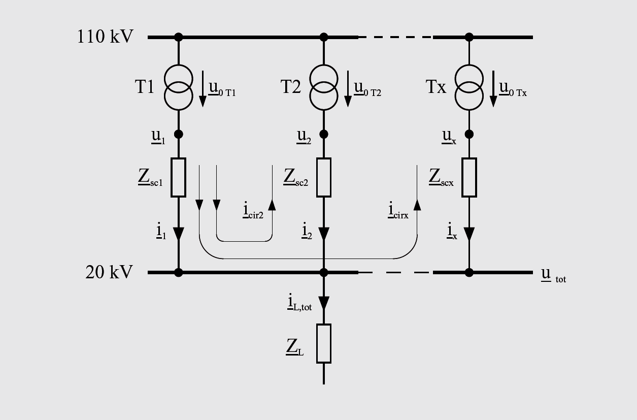
This example illustrates that the transformer T1 is additionally loaded with all of the circulating currents while all of the other transformers are relieved by their respective circulating current. Since the transformer impedances are strongly inductive and the effective component can be disregarded, such circulating currents are also called circulating reactive currents.
Even more complicating is the fact that the voltage regulation loses sensitivity, since a change in the individual open-circuit voltages u1 to ux only partially affects the total voltage of the busbar. If it is assumed that the impedances Zsc1 to Zscx are all equal and one of the transformers is upset by Δux in order to regulate the voltage, it follows that:
u’tot = u tot + Δ ux / n (4)
Equation (4) illustrates that, for example, in the case of three transformers connected in parallel (n=3) with the same impedance, a voltage variation at one transformer only affects the busbar by one-third. This circumstance greatly complicates voltage regulation. If the voltages of too highly tapped transformers are compensated for by too lowly tapped transformers, the voltage will be maximally adjusted, but circulating currents will flow. In order to be prepared for such situations, additional measured variables must be found which can be used for the parallel regulation.
Procedures for voltage regulation
REG-D® programs for parallel operation and their applications
Two decisively different types of voltage regulation are in use: Procedures which only regulate the voltage, such as the master-slave and the master-follower procedures, and those which additionally take the circulating reactive current into consideration, such as the ΔIsinϕ, ΔIsinϕ (S) and the Δcosϕ procedures. Both the applications of the parallel regulation procedures implemented in the REG-D® as well as their prerequisites are compared in Figure 8. In the following, the correct procedure for each particular task will be illustrated.
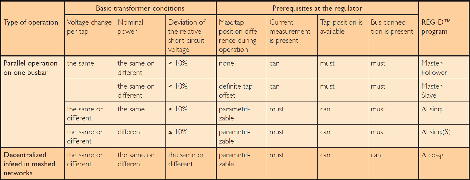
Master-slave and Master-follower procedures
These procedures regulate on the same tap positions of the transformers. In the process, one regulator takes over control while the other regulators follow its position commands (master-slave regulation). In the master-follower procedure, the slave is equipped with additional intelligence. It can actively read the tap position of the master via E-LAN and can independently position itself to match the master’s tap position. A desired tap difference existing at the beginning of the parallel regulation between the master and the slaves remains intact in the master-slave procedure. In the master-follower procedure, however, the difference is offset.
Both procedures are particularly suitable for transformers of the same construction. Transformers with differing capacities can also be operated in this manner. However, the same tap positions must then result in the same ratio (= same open-circuit voltages). In order to attain good regulation results, the relative short-circuit voltages of the transformers may not deviate too strongly (max. 10%) from each other.
Circulating reactive current procedures
In the circulating reactive current procedures, the circulating reactive current is determined by measuring the currents at the infeed of the transformers and is minimized by targeted tapping of the transformers.
ΔIsinϕ procedures
In order to maintain the circulating reactive current, it is not sufficient to simply measure the reactive current at the transformer, since this could also be due to an inductive load (refer to ix in Figure 3). In the case of two transformers operating in parallel, the circulating reactive current is the result of half of the difference between both of the measured reactive currents. The proportion caused by the load is mathematically eliminated in the process. In the case of numerous transformers, the total of all of the reactive currents is determined and is then divided by the number of transformers. As a result, the reactive current is obtained which each transformer must yield in order to cover the reactive power requirements of the load. According to Figure 3, the following is valid:
iL,tot = iT1 + iT2 + … + iTx (5)
The equations (1) through (3) have been inserted into the equation (5):
iL,tot = i1+ icir2+…+ icirx + i2 - icir2 + ix - icirx (6)
As can be seen in equation (6), all of the circulating currents are eliminated. This results in:
iL,tot = i1 + i2 … + ix (7)
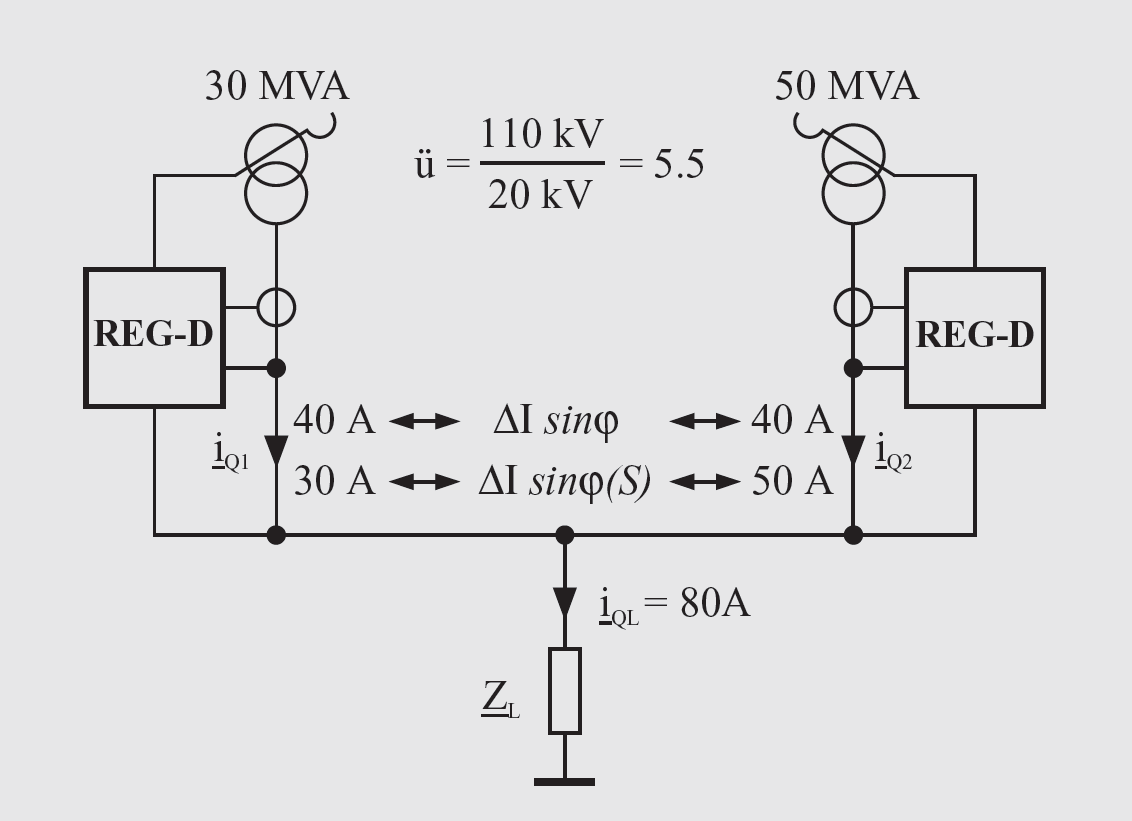
The relations in equations (5), (6), and (7) can be applied to the reactive components IQx. The sum of the load reactive currents can be calculated by adding together the reactive currents of the transformers (see Figure 4).
In order to determine the nominal reactive current per transformer, the respective reactive current must be divided by the number n of transformers. The nominal reactive current thus determined should be yielded by each transformer in order to cover the reactive power requirements of the loads. The circulating reactive current icirQx of a transformer is therefore the difference between the measured reactive current and the nominal reactive current:
icirQx = iQx - (iQ,tot · 1/n) (8)

icirQx: circulating reactive current of transformer No. x
iQx: reactive current component of transformer No. x
iQ,tot: reactive component of the total current of all of the transformers
ΔIsinϕ (S) procedures
The ΔIsinϕ(S) procedure is an expansion of the ΔIsinϕ procedure. When the nominal reactive current is calculated, the rated power of the transformers is also evaluated. This additional information makes it possible to distribute the reactive current to the transformers according to their rated power (see Figure 5).
icirQx = iQx - (iQ,tot · Sx/Stot) (9)

with:
Sx: rated power of transformer No. x
Stot: total rated power of all of the transformers
Δcosϕ procedures
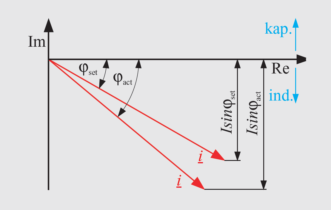
The Δcosϕ procedure has a special status among the parallel regulation programs. When several transformers feed into a widely meshed network, the regulators cannot communicate with each other via E-LAN. It is therefore not possible to mutually query the reactive currents and to mathematically calculate the circulating reactive current. The network-cosϕ (cosϕnetwork) is first determined by the operator as the setpoint. The reactive current, which results when the cosϕ at the transformer is equal to the cosϕ of the network, can be calculated from the voltage of the busbars and the transformer current voltage. If the actual reactive current is higher, the transformer is tapped lower. If the actual reactive current is lower, the transformer is tapped higher. The circulating reactive current is calculated as follows (see Figure 6):
icirQx = iTxsinϕact - iTxsinϕset (10)
Integration into the voltage regulation
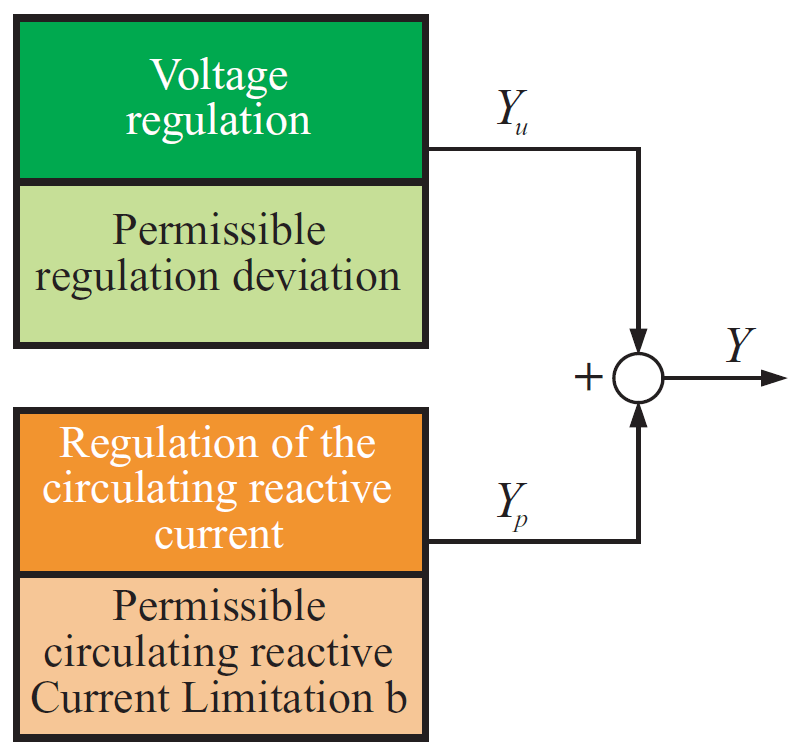
As has already been illustrated, voltage regulation is not sufficient for the regulation of transformers connected in parallel. In order to avoid circulating reactive currents, the regulation of circulating reactive currents is superimposed over the voltage regulation (Figure 7). This results in the manipulated variables Yu and Yp at:
YU = ( Uact – Uset ) / ΔUperm (11)
YP = Icir Qx / Icir Qperm (12)

with:
Uact actual value of the effective voltage
Uset setpoint of the effective voltage
ΔUperm permissible regulation deviation
Icir Qperm permissible circulating reactive current
current regulation on the voltage regulation
In addition, the following is valid for the resulting manipulated variable Y (see Figure 7):
Y = YU + YP (13)
The control commands for the regulation are derived from equation (13) as follows: for Y>+1.0, the control command LOWER will be triggered, whereas for Y<−1.0, the control command HIGHER will be triggered. Independent of each other both the voltage and circulating reactive current will be regulated to the respectively permissible deviations. Control commands which cause an impermissible change in the voltage due to minimization of the circulating reactive current are corrected via all of the transformers connected in parallel. There is therefore no remaining regulation deviation for the voltage.
The Δcosϕ procedure is also a special case in respect to the influence on the voltage regulation due to the regulation
of the circulating reactive current. There is also resulting influence when the cosϕ of the network differs from the predetermined setpoint. The remaining regulation deviation ΔU is dependent on both of the phase angles ϕset and ϕnet, on the apparent current I, on the predetermined permissible regulation deviation ΔUperm as well as on the predetermined permissible circulating reactive current IcirQperm.
ΔU=ΔUperm · (sinϕset – sinϕnet )·I / IcirQperm (14)
However, as was shown in equation 16, this influence can be limited. Along with the permissible circulating reactive current, the limitation b is given in Figure 7 as a parameter; it indicates how large yp can maximally be.
I YP I < b (15)
In this manner, the remaining regulation deviation ΔU is limited to
∆U = b · ∆Uperm (16)
In the case of strongly fluctuating loads and the resulting changes in the Network cosϕ, it is also possible to adjust the setpoint of the cosϕ through a self-learning procedure. This makes it possible to avoid regulation deviations in the voltage and impermissibly high circulating reactive currents.
Safety precautions
In all of the procedures (with the exception of the cosϕ procedure), the regulators involved in the parallel connection all exchange the necessary data via the E-LAN. If the E-LAN connection is interrupted, reliable regulation must continue to be guaranteed.
Since the Δcosϕ procedure functions without any bus connection, it is applied as an emergency program. This emergency program has been implemented as a standard in the REG-D® regulator. The operating principle can be described as follows: During undisturbed operation with the Δsinϕ and the Δsinϕ(S) procedures, the cosϕ of the network is constantly measured. After a bus failure occurs, the last measured cosϕ is interpreted as the setpoint cosϕ, and the Δcosϕ procedure will commence. When the bus failure has been corrected, the last active parallel program will be reactivated.
If there is a failure in the bus connection in the master-slave and the master-follower procedures, the slaves will automatically return to individual regulator operation. An error message will be issued to signal this condition.
Simulation software
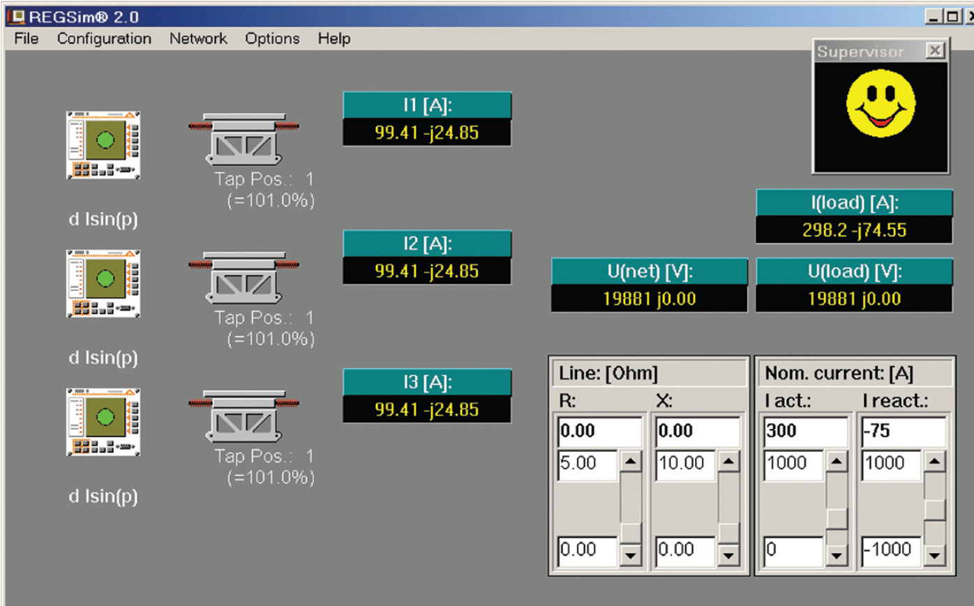
On the basis of theoretical considerations (Figure 8), it is possible to determine which parallel regulation procedure is suitable for which system. The REGSim® software (Figure 9) makes it possible to simulate parallel regulation procedures in any operating constellation with transformers, network, and loads. The regulation algorithms implemented in the regulator are applied.
Various kinds of key data (nominal voltage, transformer impedance, etc.) can be parameterized. In this manner, it is possible to simulate the REGSys® voltage regulation system in one concrete system situation. Without intervening in the real system, it is thus possible to determine how the regulation behaves in extreme situations (load surges, ground faults). The quality of the regulation (voltage stability, the number of tap changes) can already be estimated in advance. This program is, of course, also suitable for training purposes.
Automatic parallel operation
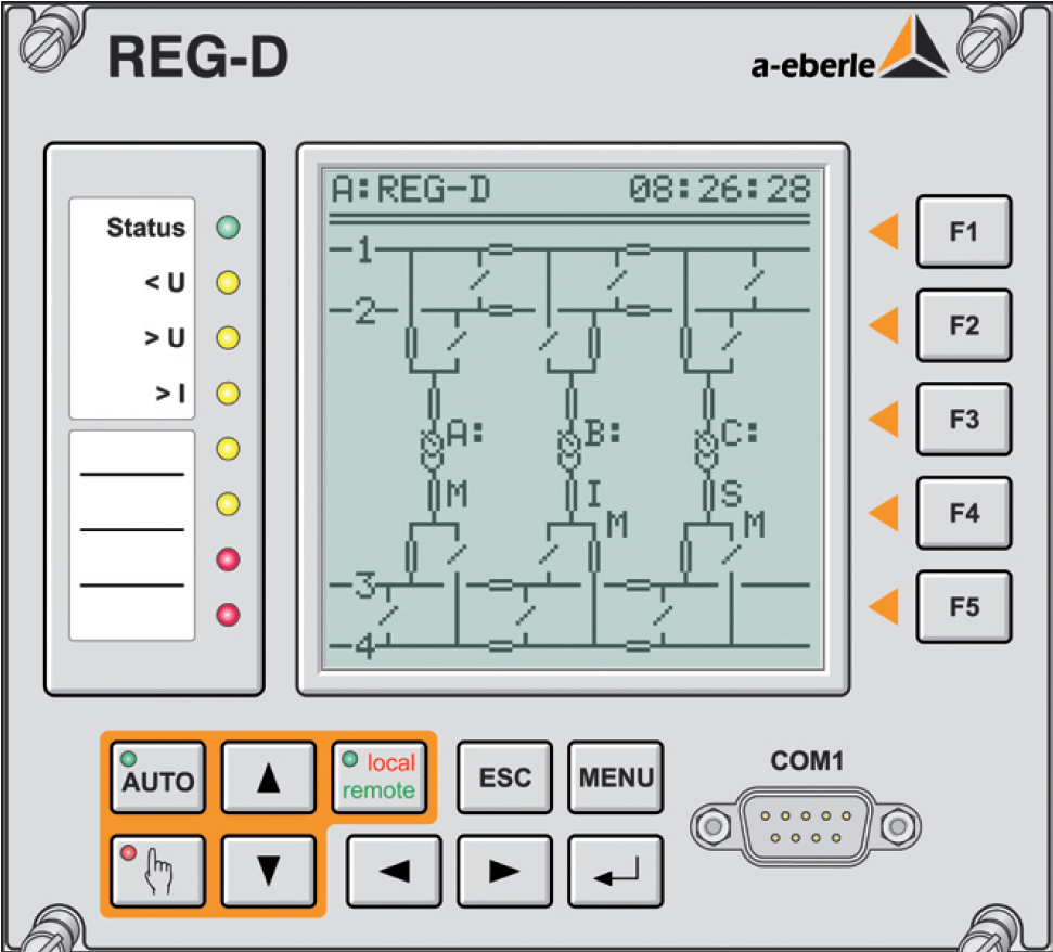
The ParaGramer (Figure 10) serves as an aid for the automatic preparation of the parallel connections and the online visualization of the operating states. The ParaGramer displays the transformers involved in the parallel operation, including the circuit-breakers, the isolators, the bus couplings, and the bus sectionalizing points in the form of a one-phase depiction. Each regulator must be supplied with a complete busbar depiction via binary inputs. On the basis of the switching states, the system automatically recognizes which transformers are fed in parallel with which other transformer(s) on one busbar. The system treats busbars connected via bus couplings as one individual busbar.
In Figure 10, for example, the transformers T1 and T3 are operating on busbar a, while transformer T2 is feeding on busbar b. With the aid of the ParaGramer, it is also possible to depict high voltage busbars. The ParaGramer is thus a suitable tool for reliably implementing the most varied parallel connections with only minimum effort.